Identifying fuel loading models (FLMs) in the field for predicting fire effects from on-site fuels
Bacciu, V.1, Pellizzaro, G.1, Scarpa, C.1
1National Research Council of Italy – Institute for the BioEconomy
Last updated: 24/09/2026
Recommended citation:
Bacciu, V., Pellizzaro, G., & Scarpa, C.. 2026. Identifying fuel loading models (FLMs) in the field for predicting fire effects from on-site fuels. In: Pere Casals, Davide Ascoli, Lena Vilà-Vilardell, Imma Oliveras, Madoka Krick (eds.) 2026. Methods handbook for characterizing fire use behavior, assessing fire effects, and monitoring soil and vegetation responses at the stand level. FIRE-ADAPT project (number 101086416), deliverable D1.1
Indicator
Fuel load: Fire behaviour models
Brief introduction
Characterizing the structural vegetation components and fuel loading is crucial for evaluating fire hazards, for the development or use of fire behavior prediction models, and for implementing decision support systems for fire management.
Fuel Loading Models (FLMs) is a classification system for predicting fire effects from on-site fuels (Lutes et al., 2009; Sikkink et al., 2009)1. Each FLM class represents fuel beds that have similar fuel loadings and produce similar fire effects. Fuel loadings include the quantities of duff, litter, fine-woody debris, and coarse woody debris (logs) in kg m–2. Fire effects include the type and amount of surface fuels consumed, the quantity of PM2.5 emissions (smoke), and the maximum soil heating obtained during combustion at 2-cm soil depth.
Managers can use FLMs to quickly estimate the fuel loads of six fuel components while in the field. FLMs can be a cost-effective alternative because fuel sampling can be done quickly or without visiting an area. FLMs can also be easily integrated with other types of plot-level data, such as stand structure or vegetation cover, to create a more comprehensive description of a plot’s characteristics with little additional field sampling (Sikkink et al., 2009).
1 For a correct identification of FLMs, users must make some coarse measurements or visual estimates of fuel load components within their sample area. For users who lack experience visually estimating fuel load, the guide provides photographs of known fuel loads to compare with plot conditions.
The guide also provides three problem sets to practice identifying FLMs from known fuel loads (Appendix J). Each example in the problem set has a photograph of on-site fuels, gives the estimated on-site fuel components, and provides step-by-step instructions to key the data to a specific FLM class (Sikking et al. 2009).
Method specifications
Method type
Soft
Hard
Method timing
Before
fire
During
fire
After fire
(short-term)
After fire
(mid-term)
After fire
(long-term)
Field skills
Low
Medium
Hard
Lab skills
Low
Medium
Hard
Material cost
Low
Medium
Hard
Time cost
Low
Medium
Hard
Calculation expertise
Low
Medium
Hard
Equipment
Plot frame: A square-meter plot frame within which fuel is assessed
Go-no-go gauge: A device including pre-cut slots of specific woody size widths
Clear plastic ruler: A ruler to be used to measure duff and litter depths if needed.
4 Double decameters
Stakes and/or pegs and hammer
Photoload procedures and sequences: Keane and Dickinson (2007) photoload sequences laminated to waterproof the pages.
Sikkink et al. (2009) guide and procedures: https://www.govinfo.gov/content/pkg/GOVPUB-A13-PURL-LPS122207/pdf/GOVPUB-A13-PURL-LPS122207.pdf
Digital camera: Pictures should be taken of the sample site and some microplot conditions for future reference.
Experimental design
Sikkink et al. (2009) do not prescribe a specific sampling scale for assessment. Citing Keane and Dickinson (2007), they emphasize that the sampling objective determines the appropriate sampling design. Highly accurate assessments rely on random or systematically stratified networks of 1 m² microplots within a sample unit. However, when the goal is a general characterization of fuels and their loadings, the estimates can be obtained at the scale of the entire sampling area (macroplot) rather than through microplots. Ideally, a 10% sample of the area is recommended, but practical constraints of time and funding often reduce this to about 1%. For instance, in a 400 m² macroplot (20 × 20 m), a 10% sample corresponds to 40 m², or 40 microplots.
Methodology
- Identify the macroareas (20 × 20 m) and install the microplots on 4 transects, 5 meters apart; the plot frame would be placed every 2 meters on each transect.
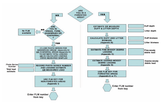
- Determine if the area is forested or non-forested. To be considered a forested area, canopy cover of trees must be greater than 10% or the habitat type should key to a forest type. Non-forested areas can consist of shrubs or grasses that are <2 m tall.
- Proceed with the FLMs identification by using the tools provided in the guide (Sikkink et al. 2009) available at https://www.govinfo.gov/content/pkg/GOVPUB-A13-PURL-LPS122207/pdf/GOVPUB-A13-PURL-LPS122207.pdf
- Forest areas:
- Estimate duff and litter depths (Appendix B of the guide)
- Pick an appropriate duff and litter bulk density value
- Calculate the duff and litter biomass
- Estimate the fine-woody debris loading: use Appendix C of the guide to determine if the fine-woody debris load is less than 0.5 kg m–2. If more precise estimates of the fine-woody component are needed, measure the 1 hr, 10 hr, and 100 hr fuels using standard fuel sampling procedures or estimate loads using the methods described in Keane and Dickinson (2007).
- Estimate log loadings (1000 hr fuels): use the photoloads (Appendix D) to decide whether you have the minimum fuel loads required in the key.
- Key to the appropriate FLM: using the values that you recorded on the plot form, follow the directions through the FLM key for forested areas. Use Appendix F.
- By compiling all the field form areas following the key in Appendix A, all the fuel load information collected in the field will help to assign the FLM that summarizes the plot’s fuel bed of the subplot.
5. Grasslands, Shrublands, or Chaparral
- Determine the cover type
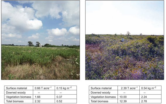
- Estimate the total fuel load on site: compare your site conditions with the photographs of known fuel loads in Appendix G (sagebrush sites) or Appendix H (non-sagebrush sites).
- Key to the appropriate FLM: use the total load determined in step 2 and match it with the load ranges in the non-forested area key (Appendix I) to pick the FLM that best describes the cover type and load estimate for your plot.
- Record the FLM number on the field form. If you need fuel-load values for individual load components to input into a software application, the median loads for each FLM are summarized in the available tables (e.g., Fig. 2).
Relation with other methods
NA
Illustrations
Data templates
NA
Further information
Lutes, D.C., Keane, R.E., Caratti, J.F., 2009. A surface fuel classification for estimating fire effects. Int. J. Wildl. Fire 18, 802–814. https://doi.org/10.1071/WF08062
Sikkink, P.G., Lutes, D.C., Keane, R.E., 2009. Field guide for identifying fuel loading models. Gen. Tech. Rep. RMRS-GTR-225. U.S. Department of Agriculture, Forest Service, Rocky Mountain Research Station, Fort Collins, CO. 33 pp.
Keane, R.E., Dickinson, L.J., 2007. The photoload sampling technique: estimating surface fuel loadings from downward-looking photographs of synthetic fuelbeds. Gen. Tech. Rep. RMRS-GTR-190. U.S. Department of Agriculture, Forest Service, Rocky Mountain Research Station, Fort Collins, CO. 44 pp.