Fuel-bed depth estimation through understory belt transects
Tardós-Ascaso, P.1; Busquets, E.1,3; Piqué, M.1,2
1Forest Science and Technology Centre of Catalonia (CTFC)
2Joint Research Unit CTFC – AGROTECNIO – CERCA, Solsona, Spain
3Agricultural Training Service. Department of Agriculture, Livestock, Fisheries and Food.
Last updated: 24/09/2026
Recommended citation:
Tardós-Ascaso P., Busquets E., Piqué M. 2026. Fuel-bed depth estimation through understory belt transects. In: Pere Casals, Davide Ascoli, Lena Vilà-Vilardell, Imma Oliveras, Madoka Krick (eds.) 2026. Methods handbook for characterizing fire use behavior, assessing fire effects, and monitoring soil and vegetation responses at the stand level. FIRE-ADAPT project (number 101086416), deliverable D1.1
Indicator
Fuel load: Surface fuel load
Brief introduction
Fuel bed depth is a key descriptor of surface fuel models. It is used to characterize straightforwardly the combined depth of the surface fuel layers, including dead and live woody fuel, herbaceous fuel and litter. It is widely used in custom fuel model development and subsequent fire behaviour modelling and determines de surface fuel bulk density and packing ratio.
Fuel bed depth is a concept open to interpretation and many estimation methods are available such as the one described in Prichard et al. (2019). The methodology described below has been refined through many years of field inventory experience and is considered an efficient and reliable approach for this estimation. Also, it easily supplements a standard dasometric inventory applied in circular plots.
Method specifications
Method type
Soft
Hard
Method timing
Before
fire
During
fire
After fire
(short-term)
After fire
(mid-term)
After fire
(long-term)
Field skills
Low
Medium
Hard
Lab skills
Low
Medium
Hard
Material cost
Low
Medium
Hard
Time cost
Low
Medium
Hard
Calculation expertise
Low
Medium
Hard
Equipment
- Measuring tapes (at least one 30 m and one 5 m)
- 3 one-meter-long ranging poles with decimetre marks
- 4 wooden, PVC or steel stake per plot
Experimental design
Forest inventory should be based on a network of sample plots distributed across the study area. The number, density, and spatial arrangement of the plots should be adapted to the characteristics of the stand, considering the variability in stand structure and forest types to ensure representative sampling. The method described below should be based on forest inventory plots, following the described principles.
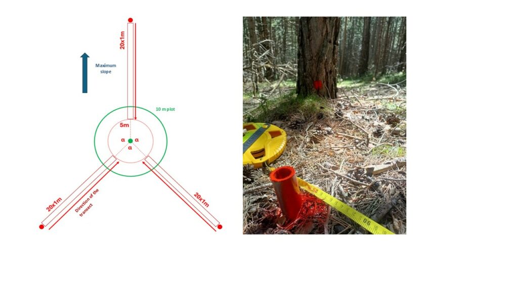
Three 20-meter linear transects are established in each plot to inventory understory components. These transects are distributed radially from the centre of the plot, maintaining a constant angle of 120° between them. The first transect (T1) should be aligned with the maximum slope ascending direction. The other two transects (T2 and T3) are located as a function of the first one, respecting the 120° angle. The starting point of each transect is located 25 meters away from the centre of the plot, measured on the ground. This point is permanently marked by driving a stake into the ground. The end point of each transect is located 5 meters away from the centre of the plot, measured on the ground, following the same radial direction as the transect. In other words, the 20-meter-long transects oriented radially from the centre of the plot are located between 25 and 5 meters from the centre of the plot (see Figure 1). This is to avoid over-representation of the centre of the plot. The transects should be defined in the field by stretching a measuring tape on the ground, as taut as possible, between the centre of the plot (meter 0) and the transect starting point (meter 25). The effective transect length, within which the different records take place, is the 20-meter section located between meter 25 and meter 5 of the measuring tape. Measurements start from the outer or initial point of the transect (meter 25) and move towards the centre of the plot to the end point of the transect (meter 5).
Methodology
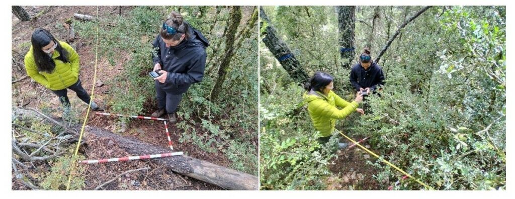
An exhaustive understory cover sampling is conducted by establishing an alternate-plot belt transect on each linear transect.Ten square 1 × 1 m plots are located on the right side of the linear transect, viewing from the starting point of the transect (meter 25) towards the centre of the main plot (meter 0). These plots are established every two meters along the linear transect, resulting in a one meter spacing between consecutive plots. The starting point of the linear transect (meter 25) corresponds to the corner of the first alternate-plot, which extends from meter 25 to meter 24. The next alternate-plot should be located between meter 23 and meter 22, leaving one square meter unsampled between adjacent plots and creating an alternate-plot belt transect. This alternate-plot method has been shown to be cost-effective in terms of sampling effort and data quality (Del Vecchio et al., 2019). The square meter within which sampling is carried out is temporarily marked on the ground using three one-meter-long ranging poles with decimetre marks (Figure 2).
The following variables are sampled within the 1 × 1 m frame of each alternate-plot:
- Shrub layer: shrub species.
- Cover by species (%)
- 2 perpendicular diameters of the crown of each shrub individual
- Maximum height by shrub individual (cm) (avoiding outliers).
- Herb layer: set of herbaceous species.
- Cover of the layer (%).
- Maximum height of the layer (cm).
- Woody debris: naturally fallen woody debris and branches.
- Cover of the layer (%).
- Maximum height of the layer (cm).
- Rock cover: presence of rocks on the surface.
- Rock cover (%).
- Bare ground: presence of exposed organic or mineral soil on the surface.
- Bare ground cover (%).
- Litter and moss: litter and moss is treated together as the upper, poorly decomposed portion of the soil organic horizon. This stratum is one of the six fuel strata described by Prichard et al. (2013). The following variables are measured:
- Cover (%)
- Litter type (coniferous or broadleaf)
- Maximum depth (cm).
Calculations
Different rules for prioritisation of the different understory components may be used to calculate fuel bed depth, which accounts for all of them. This prioritisation rule should change depending on the characteristics of the analysed stand to better represent it. Here we propose an example used in montane Pinus sylvestris stands in the Pyrenees.
In this case, fuel bed depth integrates live shrubs, woody debris, and herbaceous layer and was calculated per transect, integrating the data from each 10 square plots. Litter layer was discarded because it overlapped the other fuel layers, including herbaceous layer, showing a lower depth (around 0,8 cm). Because the sum of the covers of these three fuel components represents a multi-layer cover and may therefore exceed 100%, the three layers should be integrated into the calculation as follows:
- Calculation of the weighted mean height integrating the shrub and herbaceous layer, on each transect, using percent cover as the weighting factor. For each square plot, the proportion of the surface which is not covered by shrubs is assigned the weighted mean height of the herbaceous layer on that transect.
- Calculation of the weighted mean height integrating woody debris layer and the herbaceous layer, on each transect, using percent cover as the weighting factor. For each square plot, the proportion of the surface which is not covered by woody debris layer is assigned the weighted mean height of the herbaceous layer on that transect.
- The highest value between both weighted mean heights calculated for each transect is selected as the fuel bed depth.
Relation with other methods
The understory belt transects described below serve to obtain varied data regarding understory characteristics, that can be used to estimate the different understory components cover and height as well as the live woody fuel load following (De Cáceres et al, 2023), herbaceous fuel load following (Fernandes et al., 2012), litter and moss fuel load following (Prichard et al., 2013).
Illustrations
Further information
De Cáceres, M., & Casals, P. (2023). medfuels: Fuels of Mediterranean forests and shrublands. R package version 0.1.1.
Del Vecchio, S., Fantinato, E., Silan, G., & Buffa, G. (2019). Trade-offs between sampling effort and data quality in habitat monitoring. Biodiversity and Conservation, 28(1), 55–73. https://doi.org/10.1007/s10531-018-1636-5
Fernandes, P. M., Loureiro, C., & Botelho, H. (2012). PiroPinus: A spreadsheet application to guide prescribed burning operations in maritime pine forest. Computers and Electronics in Agriculture, 81, 58–61. https://doi.org/10.1016/j.compag.2011.11.005
Prichard, S. J., Andreu, A. G., Ottmar, R. D., & Eberhardt, E. (2019). Fuel characteristic classification system (FCCS) field sampling and fuelbed development guide. USDA Forest Service – General Technical Report PNW-GTR, 2019(GTR-972), 1–77.
Prichard, S. J., Sandberg, D. V, Ottmar, R. D., Eberhardt, E., Andreu, A., Eagle, P., & Swedin, K. (2013). Fuel Characteristic Classification System version 3.0: technical documentation. https://doi.org/10.2737/PNW-GTR-887
It is possible to add links