Skip to content

Destructive measurements combined with transects for shrub fuel load estimation

Pellizzaro, G.1,Ventura, A.1 & Arca, B.1

1National Research Council of Italy – Institute for the BioEconomy

Last updated: 25/09/2026

Recommended citation:

Pellizzaro, G.,Ventura, A. & Arca, B. 2026. Destructive measurements combined with transects for shrub fuel load estimation. In: Pere Casals, Davide Ascoli, Lena Vilà-Vilardell, Imma Oliveras, Madoka Krick (eds.) 2026. Methods handbook for characterizing fire use behavior, assessing fire effects, and monitoring soil and vegetation responses at the stand level. FIRE-ADAPT project (number 101086416), deliverable D1.1

Indicator

Fuel load: Surface fuel load

Brief introduction

Vegetation fuel is composed of various types and structures of vegetation, including herbs and shrubs. Fire behavior and characteristics can vary in relation to vegetative fuel conditions, such as dead or live fuel. Live fuel is a major component of the surface fuel in many fire-prone ecosystems, such as the Mediterranean maquis.

Several methods are available for estimating fuel load. In this case, a destructive technique is described for estimating shrub biomass and calculating the load per hectare based on species coverage percentages1. This approach involves measuring the coverage using the pinpoint intercept method, collecting samples of known volumes of fuel from individual species, drying the samples in an oven for a specified period, and weighing them to determine the dry load. Finally, the load per square meter is calculated by combining the load measurements with the specific coverage measurements.

1 This method is recommended in cases where surface fuel consists of a single or a few dominant species with compact, continuous growth and dimensions that make it easy to cut known volumes of biomass.

Method specifications

Method type

Soft

Hard

Method timing

Before
fire

During
fire

After fire 
(short-term)

After fire
(mid-term)

After fire
(long-term)

Field skills

Low

Medium

Hard

Lab skills

Low

Medium

Hard

Material cost

Low

Medium

Hard

Time cost

Low

Medium

Hard

Calculation expertise

Low

Medium

Hard
Equipment

  • 1 square frames of 1 m2 (or any other known area depending on plant size and vegetation uniformity)

  • Paper bags and ties for collecting samples

  • Pruning and garden shears to cut the vegetation

  • Scale for weighing heavy items and/or portable digital dynamometer for field weight measurements

  • A 30 meters tape and a 1 meter length pole

  • Lab scale (precision: 0.1g)

  • Lab oven

Experimental design

Establish a 15 m circular plot in each  homogeneous study area (e.g. conifer forest, mixed forest, shrubland, broadleaves forest). In each circular plot, at least three destructive samples for each species registered should be collected. Each circular plot should be marked adequately with markers and labels, and  GPS coordinates should be recorded for future samplings.

Methodology

  1. Set a central point for the 15 m radius circular plot and record the coordinates of the plot center .
  2. Establish two 30 m transects oriented North-South and East-West, intersecting at the central point of the plot.
  3. Measure vegetation cover and height along both transects. At 20 cm intervals along each transect, place a sampling pin vertically into the vegetation and record all contacts with plant species or the ground. For each contact, identify the species touching the pin and record its height. The percentage cover of each species is calculated as the number of contacts for that species divided by the total number of points along the transect.
  4. Identify the height classes present within the plot for each species (e.g. low, medium, and high)
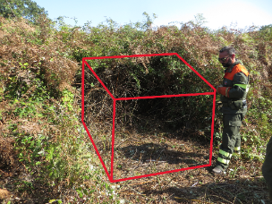
  5. For each different species and height class combination, harvest all the biomass present in a  destructive plot of at least 1 m² and place the collected material in a labelled envelope.
  6. In the laboratory, separate the fuel with a diameter greater than 6 mm from that with a smaller diameter; weigh the fresh biomass and, finally, dry the material in an oven at 102°C for 96 hours (or at 60 °C until a constant weight is reached). After drying, weigh it again to determine the dry mass.
  7. Calculate the dry weight (g m⁻²) for each species, size and height class. For all material harvested from 1 m⁻² sub-plot, the measured dry weight represents the fuel load in g m⁻².  If you have used larger subplots, you should take this into account in your calculations. For example, if you collected the material from a 4 m² subplot, you will need to divide the dry weight by 4 to obtain the live fuel load expressed in g m⁻². 
  8. To obtain the representative live fuel load for the entire plot (or area), multiply the fuel load values obtained for each species and height class by  the percentage cover (obtained from the two transects measurements), and then sum them up. 

Calculations

\mathrm{FL}\,(\mathrm{g}\,\mathrm{m}^{-2}) = \frac{ \mathrm{DW}_{\mathrm{subplot}}}{A_{\mathrm{subplot}}}
\begin{array}{l} \textbf{Where:} \\[0.5em] \mathrm{FL} = \text{Live fuel load} \\ \mathrm{DW}_{\mathrm{subplot}} = \text{Dry weight subplot} \\ \mathrm{A}_{\mathrm{subplot}} = \text{Subplot area} \end{array}

If a sub-sample of the live material from the subplot has been collected:

\mathrm{DW}_{\mathrm{subplot}}\,(\mathrm{g}) = \frac{ WW_{\mathrm{subplot}} \times DW_{\mathrm{subsample}} }{ WW_{\mathrm{subsample}} }

\begin{array}{l} \textbf{Where:} \\[0.5em] \mathrm{DW}_{\mathrm{subplot}} = \text{Dry weight subplot} \\ \mathrm{WW}_{\mathrm{subplot}} = \text{Wet weight subplot} \\ \mathrm{DW}_{\mathrm{subsample}} = \text{Dry weight subsample} \\ \mathrm{WW}_{\mathrm{subsample}} = \text{Wet weight subsample} \end{array}

Then divide the dry weight of the subplot by the total subplot area to obtain the live fuel load per square meter (g m⁻²) as shown in the first equation.

The live fuel load is calculated as the average of the all subplots.

Relation with other methods

Destructive measurements to assess shrub fuel load are often combined with other methods to assess the fuel load of other components (e.g., dead woody fuel, litter, duff).

To combine fuel load and bulk density measurements, simply add the following:

Ideally, before cutting, partition the subsample into 16 quadrants. Measure the plant height in each quadrant as the vertical average distance from the soil surface to the top of the branches of the predominant species in that quadrant. Calculate the volume by multiplying the average height obtained in the 16 quadrants by the area of the subplot. To calculate the bulk density (g m⁻³) of each subplot, divide the total dry mass by the volume.

Illustrations

Subplot before cutting
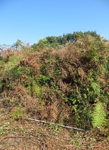
Subplot after biomass cutting

Data templates

NA

Further information

Catchpole, W.R. & Wheeler, C.J. (1992). Estimating plant biomass: a review of techniques. Australian 

Journal of Ecology 17: 121-131.

Lutes, Duncan C.; Keane, Robert E.; Caratti, John F.; Key, Carl H.; Benson, Nathan C.; Sutherland, Steve; Gangi, Larry J. 2006. FIREMON: Fire effects monitoring and inventory system. Gen. Tech. Rep. RMRS-GTR-164. Fort Collins, CO: U.S. Department of Agriculture, Forest Service, Rocky Mountain Research Station. 1 CD.