Photoload sampling technique for surface downed dead woody fuel estimation
Bacciu, V.1, Scarpa, C.1, Pellizzaro, G.1
1National Research Council of Italy – Institute for the BioEconomy
Last updated: 24/09/2026
Recommended citation:
Bacciu, V., Scarpa, C., & Pellizzaro, G. 2026. Photoload sampling technique for surface downed dead woody fuel estimation. In: Pere Casals, Davide Ascoli, Lena Vilà-Vilardell, Imma Oliveras, Madoka Krick (eds.) 2026. Methods handbook for characterizing fire use behavior, assessing fire effects, and monitoring soil and vegetation responses at the stand level. FIRE-ADAPT project (number 101086416), deliverable D1.1
Indicator
Fuel load: Surface fuel loading
Brief introduction
Fuel loading is essential for assessing fire hazards, developing fire behaviour predictive models, evaluating the impacts of alternative fuels and treatments to protect lives and ecosystems, and implementing decision-support systems for fire management. Measuring surface fuel loadings in the field is challenging because it requires a complex integration of several sampling methods designed for different scales (Keane and Dickinson, 2007).
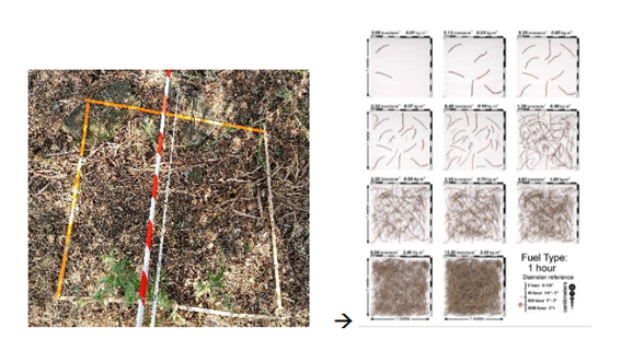
The photoload sampling technique is a method to quickly and accurately estimate loadings for six common surface fuel components (1 hr, 10 hr, 100 hr, and 1000 hr downed dead woody1 fuels), based on Keane and Dickinson (2007) approach. This method consists of visually comparing fuel conditions in the field with photoload sequences to estimate fuel loadings (Figs. 1 and 2).
The photoload technique specifically identifies five fuel components:
- 1 hour: <6 mm diameter downed, dead, woody fuels
- 10 hour: 6-25 mm diameter downed, dead, woody fuels
- 100 hour: 2.5-7.5 cm diameter downed, dead, woody fuels
- Shrub: Dead and live shrubby fuels
- Herb: Dead and live grass and forb fuels
Here we describe the methodology for measuring dead downed woody fuel components.
Method specifications
Method type
Soft
Hard
Method timing
Before
fire
During
fire
After fire
(short-term)
After fire
(mid-term)
After fire
(long-term)
Field skills
Low
Medium
Hard
Lab skills
Low
Medium
Hard
Material cost
Low
Medium
Hard
Time cost
Low
Medium
Hard
Calculation expertise
Low
Medium
Hard
Equipment
Plot frame: A square meter plot frame with the square meter area measured on the inside dimensions of the frame.
Go-no-go gauge: A device that has the widths of each woody size class upper diameter range.
Clear plastic ruler to estimate log diameters and branch lengths. It can also be used to measure duff and litter depths if needed.
4 Double decameters
Stakes and/or pegs and hammer
Photoload procedures and sequences: Photoload sequences laminated to waterproof the pages (Keane and Dickinson, 2007).
Digital camera: Pictures should be taken of the sample site and some microplot conditions for future reference
Experimental design
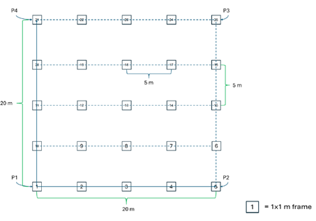
According to Keane and Dickinson (2007), the sampling objective determines the appropriate sampling design. Highly accurate assessments rely on random or systematically stratified networks of 1 m² microplots within a sample unit. Ideally, a 10% sample of the area is recommended, but practical constraints of time and funding often reduce this to about 1%. For instance, in a 400 m² macroplot (20 × 20 m), a 10% sample corresponds to 40 m², or 40 microplots. The following experimental design has been designed under the premises of the DRYAD Horizon Europe project (https://dryad-project.eu/). Within several sampling areas, rectangular grids were established for a total of 25 microplots each.
Methodology
- Define the sampling area. Create a rectangular grid established through orthogonal transects, with P1, P2, P3 and P4 as the reference points located at the outer corners of the square
- Establish the main transects. From the vertices P1–P2 and P1–P4, lay out the main transects as guiding lines along the area’s sides (Fig. 1).
- Create the grid. Use the main transects to draw parallel internal lines, which delineate the grid of the sampling points, named micro-plots
- Place the stakes. Starting from the main reference point, place a stake every 5 meters to create and mark the grid. To ensure a correct alignment of the stakes, use double decameters
- Position the micro-plots. At regular 5-meter intervals, position a 1×1 m frame for each micro-plot within the grid (Fig. 2).
Estimating the downed dead fuel load
6. For each microplot 1×1 m, the operator must estimate downed dead fuel loading by matching one or more of the photoload sequences in Appendix A (Keane and Dickinson, 2007).
7. In the case of slash and activity fuelbeds, adjust the loading for fuelbed depth for the component. First, select the photoload picture that best matches the top of the fuelbed (point 6). Then measure with a ruler the average fuelbed depth and the maximum diameter of the woody fuel class. Adjusted fuel load = Photoload estimate × Fuelbed depth ÷ maximum diameter of the woody fuel class.
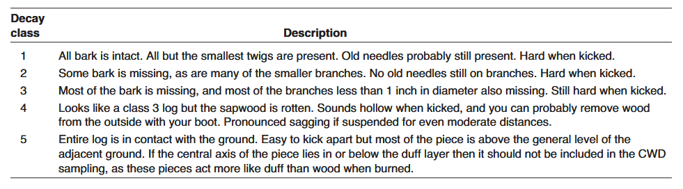
8. Evaluate the degree of decay for downed woody fuels (100 hr and 1000 hr logs). The degree of decay for downed woody fuels can also influence the accuracy of fuel load estimates, and adjustments should be made to correct for the amount of rot. The photoload sampling technique assumes all downed dead woody fuel is sound. So, any observed decay will reduce the loading estimates.
9. Measure the diameter of large woody fuels (100 hr and 1000 hr logs, >2.5 cm). The range of diameters in large woody fuels is so large that photographs depicting a loading for the fuels with diameters at the small end of the size class may underestimate loadings by a factor of nine for 100 hr fuels because loading increases by the square of the diameter.
10. Take photos of the vegetation inside the 1×1 meter frames.
Calculations
In the case of slash and activity fuelbeds, the component loading must be adjusted for fuelbed depth.
First, select the photoload picture that best matches the top of the fuelbed.
Then measure with a ruler the average fuelbed depth and the maximum diameter of the woody fuel class.
\mathrm{FL}(\mathrm{kg}\,\mathrm{m}^{-2})= \text{Photoload estimate} \times \frac{FD}{D_{\mathrm{max}}}
Example for a slash bed composed of a 10 hour woody fuelbed that is 10 cm deep and matching with the photoload picture of 5 kg m–2:
Photoload estimate = 5 kg m–2
Fuelbed depth = 0.10 m
Maximum fuel diameter = 0.025 m
\mathrm{FL}(\mathrm{kg}\,\mathrm{m}^{-2})= 5 \times \frac{0.10}{0.025} = 20\, \mathrm{kg}\,\mathrm{m}^{-2}
Degree of decay for downed woody fuels adjustment (Lutes et al., 2006, Fig. 3):
- Decay class 1: No need to adjust for decay
- Decay class 2: No need to adjust for decay
- Decay class 3: Multiply loadings by a factor of 0.90
- Decay class 4: Multiply loadings by a factor of 0.75
- Decay class 5: Multiply loadings by a factor of 0.50
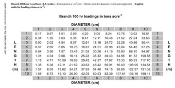
Large woody fuel adjustments (>100 hr, diameter > 2.5 cm): Use the table provided by Keane and Dickinson (2007). The following steps are used to estimate loading using the tables:
- Measure the length of all woody fuel particles in the >100 hr fuel component within the microplot (1 m-2). This can be visually estimated or actually measured using a cloth tape.
- Estimate the average diameter across all logs within the microplot. The best estimates of average diameter are done using the quadratic mean square estimate where the sum of the squares of all woody fuel particles are estimated and then divided by the number of particles and then the square root is taken.
- In the table in Fig 4, find the loading by cross-referencing the length and diameter.
- Use linear extrapolation across rows or columns if the diameter or lengths do not match the categories listed in the table
- Record the final loading on the plot sheet
Relation with other methods
The plot design can be also useful to estimate the Herbaceous fuel load
Illustrations
Data templates
NA
Further information
Keane, Robert E.; Dickinson, Laura J. 2007. The photoload sampling technique: estimating surface fuel loadings from downward-looking photographs of synthetic fuelbeds. General Technical Report RMRS-GTR-190. Fort Collins, CO: U.S. Department of Agriculture, Forest Service, Rocky Mountain Research Station. 44 p. https://research.fs.usda.gov/treesearch/26755
DRYAD Protocol for the fuel estimate, sampling and characterization University of Sassari and CNR-IBE V. 27.10.2025
Sikkink, Pamela G.; Lutes, Duncan C.; Keane, Robert E. 2009. Field guide for identifying fuel loading models. Gen. Tech. Rep. RMRS-GTR-225. Fort Collins, CO: U.S. Department of Agriculture, Forest Service, Rocky Moun tain Research Station. 33 p
Lutes, Duncan C.; Keane, Robert E.; Caratti, John F.; Key, Carl H.; Benson, Nathan C.; Sutherland, Steve; Gangi, Larry J. 2006.
FIREMON: Fire effects monitoring and inventory system. Gen. Tech. Rep. RMRS-GTR-164-CD. Fort Collins, CO: U.S.
Department of Agriculture, Forest Service, Rocky Mountain Research Station. 1 CD. https://www.researchgate.net/publication/228690001_FIREMON_Fire_effects_monitoring_and_inventory_system