Skip to content

Photos and destructive sampling for estimating fuel load and volume of shrubs

Bacciu, V.1, Pellizzaro, G.1, Scarpa, C.1

1National Research Council of Italy – Institute for the BioEconomy

Last updated: 24/09/2026

Recommended citation:

Bacciu, V., Pellizzaro, G., & Scarpa, C. 2026. Photos and destructive sampling for estimating fuel load and volume of shrubs. In: Pere Casals, Davide Ascoli, Lena Vilà-Vilardell, Imma Oliveras, Madoka Krick (eds.) 2026. Methods handbook for characterizing fire use behavior, assessing fire effects, and monitoring soil and vegetation responses at the stand level. FIRE-ADAPT project (number 101086416), deliverable D1.1

Indicator

Fuel flammability: Fuel structure

Brief introduction

Characterizing the structural vegetation components and fuel loading is crucial for evaluating fire hazards, for the development of fire behavior predictive models, and for implementing decision support systems for fire management. To predict fire behavior and spread through different plant communities, it is important to have an estimation of the bulk density of the different vegetation components (from tree canopies to understory layers). 

Bulk density (kg m–3) is the mass of a fuel component divided by the total volume of the space in which it resides (Keane 2015). It is a convenient measure of fuelbed compactness (McCaw, 1991b). For instance, in Rothermel‘s (1972) fire spread model, fuelbed compactness (dimensionless) is the fraction of fuel bed occupied by fuel and is calculated from the ratio of fuel bed bulk density (ρb) to particle density (ρp), where (ρb) is the dry fuel mass per unit fuel-bed volume and (ρp) is the dry fuel mass per unit volume of the fuel particles. . In modelling studies, particle density is usually assumed as a constant; therefore, fuelbed bulk density is equivalent to compactness. Fuelbed bulk density is determined from estimates of fuel loading and fuelbed depth, which is an estimate of the vertical extent of the combustion zone (Brown, 1981). When the fuel is compact, it is common to observe slower fire spread rates (Biswell, 1989). Fuels with a smaller compactness react faster to moisture changes and have more oxygen for the combustion process.
Method specifications

Method type

Soft

Hard

Method timing

Before
fire

During
fire

After fire 
(short-term)

After fire
(mid-term)

After fire
(long-term)

Field skills

Low

Medium

Hard

Lab skills

Low

Medium

Hard

Material cost

Low

Medium

Hard

Time cost

Low

Medium

Hard

Calculation expertise

Low

Medium

Hard

Equipment

  • Poles

  • Paper bags and ties for collecting samples

  • Pruning and garden shears to cut the vegetation

  • Scale for weighing heavy items

  • A decameter of 30 meters and a rigid meter

  • A camera

Experimental design

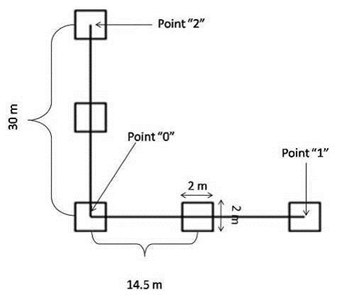
The fuel load and volume of shrubs are estimated through fixed-area plots, secondary units of the cluster sampling approach (Corona, 2000). The plots (sample units 2×2 m) are placed in proximity to each other across two linear transects disposed orthogonally. The orthogonal disposition of the transects permits sampling along two orthogonal guides, avoiding the possible bias due to topographic pattern. The transect length may vary according to several factors, including the minimum size of the sampling area and environmental characteristics. Transect and plot coordinates are recorded with a GPS for future sampling. 

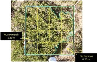
The fuel load can be estimated by complete destructive sampling methodology or double sampling methodology. Cover and height of species are collected within the plot, ideally partitioned into 16 quadrants.

Methodology

  1. Identify the location of the cross point of two linear transects: set the central point, mark the coordinates (point 0).
  2. Trace two transects of 30 m length directed North-South and East-West, intersecting the central point. The transects are disposed orthogonally, the final transect points are recorded with a GPS, and called point 1 and point 2. The measuring tape is stretched straight above the vegetation canopy. 
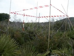
  3. Along the transects, five plots (2×2 m) are placed at an equal distance of 14.5 m from each other. Their centres were recorded with the GPS, and the boundaries were defined with tape and poles
  4. Cover measurements: For each sampling plot, several digital photos are collected by placing a digital camera with remote control perpendicular to the ground at about two meters above the plants. The images are imported and analysed to calculate the area covered by each species; the plot perimeter and the perimeter of each species within the plot are digitised, and the cover area is then computed.
  5. Height measurements: ideally, each plot is partitioned into 16 quadrants. In each quadrant, plant height is measured within the plot as the vertical average distance from the soil surface to the top of the branches of the predominant species of each quadrant.
  6. Fuel load measurements: All plant material within each plot is clipped at ground level, separated by species, weighed in the field, and bagged for subsequent laboratory analysis. In the laboratory, shrub biomass is weighed fresh, then oven-dried at 102 °C for 96 hours. After drying, the material is weighed again to determine dry mass. PS: If the live material collected in the field by the subplot is very abundant, select a sub-sample (about 20% of the total weight) and insert it in the oven.
  7. To calculate the bulk density (kg m–3) of each plot, the total dry mass is divided by the volume. Volume is calculated by multiplying the average height obtained within the 16 quadrants by the area covered by the vegetation.

Calculations

\mathrm{BD}\,(\mathrm{kg}\,\mathrm{m}^{-3})= \frac{W_d}{V}

\begin{array}{l} \textbf{Where:} \\[0.5em] \mathrm{BD} = \text{Bulk density} \\ W_d = \text{Total dry weight (kg)} \\ V = \text{Volume } (\mathrm{m}^{3}) \end{array}
\mathrm{V}(\mathrm{m}^{3})= \bar{H} \times A_{\mathrm{veg}}
\begin{array}{l} \textbf{Where:} \\[0.5em] \mathrm{V} = \text{Volume} \\ \bar{H} = \text{Average height across the 16 quadrants (m)} \\ A_{\mathrm{veg}} = \text{Area covered by vegetation }(\mathrm{m}^{2}) \end{array}

Relation with other methods

NA

Illustrations

Set up of two linear transects and sampling units (plots)
Example of sampling plot
Species, cover, and heights in the 16 plot quadrants

Data templates

NA

Further information

McCaw W.L., 1991b. Measurement of fuel quantity and structure for bushfire research and management. In Conference on bushfire modeling and fire danger rating systems. Canberra. (eds. N.P. Cheney and A.M. Gill) pp. 147-156. (CSIRO)

Rothermel R.C., 1972. A Mathematical Model for Predicting Fire Spread in Wildland Fuels. USDA Forest Service Research Paper, INT-115. Ogden, UT: Intermountain Forest and Range Experiment Station.

Brown J.K., 1981. Bulk densities of nonuniform surface fuels and their application to fire modeling. Forest Science 27, 667-783.

Biswell H.H., 1989. Prescribed Burning in California Wildlands Vegetation. Berkeley, CA: University of California Press.